关于pytorch-profile的二三事。相较于使用C和Nvidia的相关profile工具,感觉包装之后使用pytorch-profile工具进行分析也是一个可取之处。
profile with autograd
首先是一个简单的CUDA计时工具:
def time_pytorch_function(func, input):
    # CUDA IS ASYNC so can't use python time module
    start = torch.cuda.Event(enable_timing=True)
    end = torch.cuda.Event(enable_timing=True)

    # Warmup
    for _ in range(5):
        func(input)

    start.record()
    func(input)
    end.record()
    torch.cuda.synchronize()
    return start.elapsed_time(end)
如果仅仅是使用time进行相关操作的画,实际上记录的只是启动CUDA核函数所需要的时间,因此合理的记录需要使用cuda.Event操作来进行详细的记录。
但是即便如此,上面的计时工具也过于简单,在实际的场景中是需要知道各个部分所需要的时间的,这时候就可以使用第一步,pytorch autograd profile
with torch.autograd.profiler.profile(use_cuda=True) as prof:
    torch.square(b)

print(prof.key_averages().table(sort_by="cuda_time_total", row_limit=10))
使用并不复杂,上述代码的输出如下:
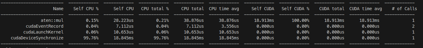
这个东西会展示代码内核的所有过程以及其花费的时间(这里有一个注意的就是Square实际上使用的是乘法实现的,这个之后再说吧)
pytorch profiler
这个东西是一个可视化的分析工具,有点类似于nvidia-profile工具,其会生成一个json文件,可以在浏览器中打开并查看,其视图如下:
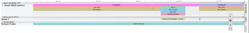
其使用方式倒也很简单,从简单的来看的话实际上只有如下步骤:
import torch
from torch.profiler import profile, record_function, ProfilerActivity


## Default way to use profiler
with profile(activities=[ProfilerActivity.CPU, ProfilerActivity.CUDA]) as prof:
    for _ in range(10):
        a = torch.square(torch.randn(10000, 10000).cuda())
prof.export_chrome_trace("trace.json")
当然考虑到实际场景可能会需要一些预热、重复等操作,可以使用如下版本:
with torch.profiler.profile(
    activities=[
        torch.profiler.ProfilerActivity.CPU,
        torch.profiler.ProfilerActivity.CUDA,
    ],

    # In this example with wait=1, warmup=1, active=2, repeat=1,
    # profiler will skip the first step/iteration,
    # start warming up on the second, record
    # the third and the forth iterations,
    # after which the trace will become available
    # and on_trace_ready (when set) is called;
    # the cycle repeats starting with the next step

    schedule=torch.profiler.schedule(
        wait=1,
        warmup=1,
        active=2,
        repeat=1),
    on_trace_ready=trace_handler
    # on_trace_ready=torch.profiler.tensorboard_trace_handler('./log')
    # used when outputting for tensorboard
    ) as p:
        for iter in range(10):
            torch.square(torch.randn(10000, 10000).cuda())
            # send a signal to the profiler that the next iteration has started
            p.step()
然而实际上上述的工具并不能提供给我们更加详细的相关内容以帮助我们实现更好的优化,但是一个可能的方法是通过查看源码比较来实现对核函数的更好理解,具体的可以在pytorch的代码仓库中找到:
ncu Nvidia-cuda profile
ncu是个非常神奇的东西,相较于nvidia基于java的profile工具,这个工具同样能提供足够多的信息以帮助优化或者理解,其使用方式也非常容易:
ncu python xxx.py
其将会把整个过程中的各个core以及对应的性能指标都进行输出,甚至能提供一个理想的峰值,只可惜支持的显卡相当有限。
CPP bind for pytorch
在进行内核编写的时候,如果想要方便的被pytorch和python所使用,还需要使用诸如pybind等操作来实现接口的调用,在某种程度上来说不算太过复杂,但是实际上pytorch有自己的构建方式:torch.utils.cpp_extension,一段实例代码如下:
import torch
from torch.utils.cpp_extension import load_inline

# Define the CUDA kernel and C++ wrapper
cuda_source = '''
__global__ void square_matrix_kernel(const float* matrix, float* result, int width, int height) {
    int row = blockIdx.y * blockDim.y + threadIdx.y;
    int col = blockIdx.x * blockDim.x + threadIdx.x;

    if (row < height && col < width) {
        int idx = row * width + col;
        result[idx] = matrix[idx] * matrix[idx];
    }
}

torch::Tensor square_matrix(torch::Tensor matrix) {
    const auto height = matrix.size(0);
    const auto width = matrix.size(1);

    auto result = torch::empty_like(matrix);

    dim3 threads_per_block(16, 16);
    dim3 number_of_blocks((width + threads_per_block.x - 1) / threads_per_block.x,
                          (height + threads_per_block.y - 1) / threads_per_block.y);

    square_matrix_kernel<<<number_of_blocks, threads_per_block>>>(
        matrix.data_ptr<float>(), result.data_ptr<float>(), width, height);

    return result;
    }
'''

cpp_source = "torch::Tensor square_matrix(torch::Tensor matrix);"

# Load the CUDA kernel as a PyTorch extension
square_matrix_extension = load_inline(
    name='square_matrix_extension',
    cpp_sources=cpp_source,
    cuda_sources=cuda_source,
    functions=['square_matrix'],
    with_cuda=True,
    extra_cuda_cflags=["-O2"],
    build_directory='./load_inline_cuda',
    # extra_cuda_cflags=['--expt-relaxed-constexpr']
)

a = torch.tensor([[1., 2., 3.], [4., 5., 6.]], device='cuda')
print(square_matrix_extension.square_matrix(a))
注意这里有一些有趣的选项:build_directory可以让你将代码生成到指定目录,此外,直接使用CPP的好处就是不需要使用多个文件或者文件夹来方式库文件、接口文件等等,因此可以减少复杂程度。这也算的上是一种新的pytorch调用方式,只不过每次都需要编译(X
triton first
相较于直接使用CUDA暴力编写和尝试加速,这往往并不是一个较好的手段(尤其是考虑到C编程的复杂程度和接口的复杂程度),从CUDA直接到应用阶段的不断调优是需要根据各种性质来进行的,而CUDA无法很好的屏蔽掉这一点,因此可以考虑先从triton入手进行编写和优化(更何况triton直接生成机器码)只可惜比较幽默的是我的笔记本同样带不动triton(其最小的计算能力也得达到7.0)
但是使用triton还是有坏处的,一个较大的一点就是因为缺少内存管理导致实际上还有诸多地方进行优化(众所周知,内存是CUDA的一个重要部分),但是对于学习CUDA确实是一个不错之选。
@triton.jit
def square_kernel(output_ptr, input_ptr, input_row_stride, output_row_stride, n_cols, BLOCK_SIZE: tl.constexpr):
    # The rows of the softmax are independent, so we parallelize across those
    row_idx = tl.program_id(0)
    # The stride represents how much we need to increase the pointer to advance 1 row
    row_start_ptr = input_ptr + row_idx * input_row_stride
    # The block size is the next power of two greater than n_cols, so we can fit each
    # row in a single block
    col_offsets = tl.arange(0, BLOCK_SIZE)
    input_ptrs = row_start_ptr + col_offsets
    # Load the row into SRAM, using a mask since BLOCK_SIZE may be > than n_cols
    row = tl.load(input_ptrs, mask=col_offsets < n_cols, other=-float('inf'))

    square_output = row * row

    # Write back output to DRAM
    output_row_start_ptr = output_ptr + row_idx * output_row_stride
    output_ptrs = output_row_start_ptr + col_offsets
    tl.store(output_ptrs, square_output, mask=col_offsets < n_cols)


def square(x):
    n_rows, n_cols = x.shape
    # The block size is the smallest power of two greater than the number of columns in `x`
    BLOCK_SIZE = triton.next_power_of_2(n_cols)
    # Another trick we can use is to ask the compiler to use more threads per row by
    # increasing the number of warps (`num_warps`) over which each row is distributed.
    # You will see in the next tutorial how to auto-tune this value in a more natural
    # way so you don't have to come up with manual heuristics yourself.
    num_warps = 4
    if BLOCK_SIZE >= 2048:
        num_warps = 8
    if BLOCK_SIZE >= 4096:
        num_warps = 16
    # Allocate output
    y = torch.empty_like(x)
    # Enqueue kernel. The 1D launch grid is simple: we have one kernel instance per row o
    # f the input matrix
    square_kernel[(n_rows, )](
        y,
        x,
        x.stride(0),
        y.stride(0),
        n_cols,
        num_warps=num_warps,
        BLOCK_SIZE=BLOCK_SIZE,
    )
    return y
pytorch spend time on where?
主要有如下几部分:
- python处理
- 数据结构构建和分配对应的Tensor
- 数据读写
- GPU计算
- kernel启动时间
- 内存访问读写(重大开销)
- 实际计算时间(重大开销)
相较于使用一步一步进行计算的过程,pytorch逐步进行着操作融合的改进,比如说:
%timeit gelu(x);
%timeit torch.nn.functional.gelu(x)
前者是自定义的gelu函数,后者是torch自带的,相较于自定义的函数,torch自带的尽可能在内核中完成所有的操作而不是一个一个操作进行
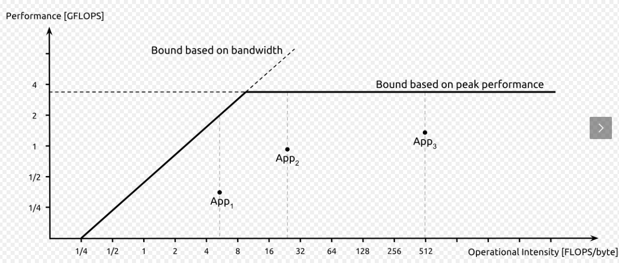
roofline model用于权衡带宽和计算速度的在理想情况下的最大值,通常情况下可以通过隐蔽延迟的方式进行提速
pytorch CUDA
主要在torch.cuda中的一些设置,其中非常常见的是一些设备的设置,此外还有一些很细节的设置:
torch.backends.cuda.matmul.allow_tf32 = self.train_config.use_amp
torch.backends.cudnn.allow_tf32 = self.train_config.use_amp
这里是使用Tensor Core进行矩阵乘法、卷积的计算,但是问题在于tensor core是半精度的,对于全精度的计算会有一定的精度损失。AMP
Optimizing optimizer
首先,在了解优化器之前,如何对多维数组实现快速的计算?
-
最直观就是传vector,但是CUDA不支持
-
ppt给出这样一个例子:对于单个数字的add操作或许可以直接进行,但是对于数组(多维Tensor)而言,应该如何使用CUDA实现?通常来说最简单直接的方式就是将所有的数组转换成向量,之后通过二维指针的形式传输到CUDA内核中。然而这种方式完全错误,传入二维指针之后,很显然,CUDA是无法获取其中的一维数据的,因此会导致引用出错(因为这些数据还在CPU上),因此,合理的方式是传引用?但是注意,C还没有引用这个东西
-
可以尝试使用结构体包装三个数组进去然后传入到kernel。但是由于CUDA参数空间限制为4KB因此会出现错误
-
使用批处理,多次处理3方法即可:但是这种方法也会带来问题,一个较大的影响就是当数据量极大时,需要使用大量的CUDA内核启动开销。
- 结合批处理和内存拷贝,把2和4进行合并即可。因此可以通过现对数据进行分块再打包从而实现高效的计算。
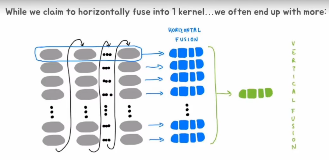
上述就是目前pytorch优化器的一种实现,很显然,上述的实现其实是相当繁琐的,在进行部分数据运算时需要大量的操作进行数据的处理和划分从而满足并行计算的需求。因此更好的操作是让pytorch能够自动识别数据的格式和运算的方式,自动化的完成上述工作,这就是接下来要提出的torch.compile的实现了。
虽然上面讲了这么多,但是torch.compile实际上解决的是垂直融合,即将垂直方向上的操作进行fusing从而提高性能而不是水平融合
Performence CheckList
其实PPMP书中对于CUDA的性能已经有了较为详细的说明,考虑到CUDA计算的架构复杂度,很多地方其实更倾向于通过案例来说明优化策略,这也是这一章节所想要说明的。主要分为以下几个部分:
- 合并内存访问
- 最大化使用率
- 判断是内存瓶颈还是计算瓶颈
- 最小化控制流分支
- 填充重用的数据(或者说分块)
- 私有化
- 粗线程块
- 从数学角度提高计算性能
合并内存访问
首先,对于CUDA编程而言的一个核心其实是理解存储模型。不同的访存所需要的延迟时间不同,对于,不过通常来说有shared « L1 < L2 « global。
此外,无论是网络或者计算,在讨论带宽时,不可避免的会遇到延迟的问题,由于这是由物理结构决定的,因此无论如何都无法减少延迟而只能实现隐藏延迟。
占用率
瓦片量化:当矩阵维度与线程块维度不能被整除
波量化:所有的相乘块数量不能被SM块整除
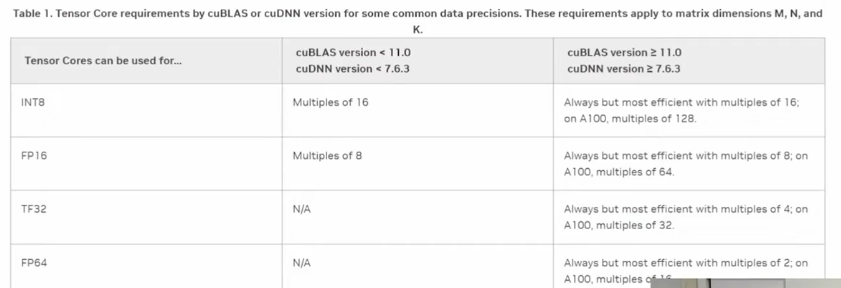
因此上述问题也会导致TensorCore的计算效率,比如:
占用率的核心其实就是调整Block和Grid的大小使得其整体使用率提升,但是通常情况下需要多种场景下的测试,这时就有一个非常好的CUDA函数来实现上述功能:cudaOccupancyMaxPotentialBlockSize()这个函数会返回用户推荐的block size和grid size来取得最佳的效果。
判断是内存瓶颈还是计算瓶颈
前面已经提到了roofline模型,然而实际上对于计算的瓶颈是可以根据计算强度、数据格式判断的。一个鲜明的例子就是对于8位和32位,相较于32位数据,8位数据可以通过每次进行4次运算来实现更好的内存占用,从而实现更快地速度,这也就是为什么量化非常重要。
对于带宽受限的kernel,通常解决方法就是:Fuse(FlashAttention), 各种量化手段,编译
而对于计算受限的kernel,一般来说解决方案就是写更好的方法来实现。
填充重用的数据(或者说分块)
通过将数据放到共享内存从而实现更高的速度,应用场合算是比较多了。
从实现角度来讲,分块是个复杂的技巧,但是通常来说本质上就是一个四层for循环
最小化控制流分支
线程束内的代码在遇到判断条件时由于分支不同导致结果不同,从而使得部分线程拖后腿影响整体性能(线程发散以指数倍进行),这里代码给了一个非常巧妙地实现可以用来学习:
__global__ void processArrayWithDivergence(int *data, int N) {
    int idx = blockIdx.x * blockDim.x + threadIdx.x;
    if (idx < N) {
        if (data[idx] % 2 == 0) {
            data[idx] = data[idx] * 2;
        } else {
            data[idx] = data[idx] + 1;
        }
    }
}

__global__ void processArrayWithoutDivergence(int *data, int N) {
    int idx = blockIdx.x * blockDim.x + threadIdx.x;
    if (idx < N) {
        int isEven = !(data[idx] % 2);
        data[idx] = isEven * (data[idx] * 2) + (!isEven) * (data[idx] + 1);
    }
}
线程粗化
听起来很复杂,实际上就是让每个线程多处理几个元素(当然,通常会有更加复杂的限制条件和写法
私有化
在进行写入全局数据和共享数据之前先更新数据(减少数据读取),其实也和分块类似
从数学角度提高计算性能
典型的设计就是softmax和flashattention
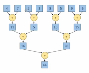
Reduction
归约,这个倒是不复杂,利用分治+洗牌操作来求和或者求最值等时非常好用,当然也会存在一些细节。
对于浮点数计算,由于浮点数计算不满足加法交换律,所以问题就导致结果不唯一,为了保证结果稳定性,一个可行的方法就是采用一个参数:
torch.use_deterministic_algorithms(True)
基本而言原理是强制一定程度的同步,但是问题在于这种同步会导致性能的下降。举个例子:
[1e-20] * 10 + [1e20, -1e20]
上述列表如果从左往右计算求和时,结果为0.0但是从右往左时结果为9.9xxxx7e-19,这就是由于计算时的浮点数溢出导致的。
归约虽然简单实用,但是也存在着相当夸张的问题。首先,显然的,会导致线程diversage从而极大的降低性能,下面是两个测试代码:
__global__ void FixDivergenceKernel(float* input, float* output) {
    unsigned int i = threadIdx.x; //threads start next to each other
    for (unsigned int stride = blockDim.x; stride >= 1; stride /= 2) { // furthest element is blockDim away
        if (threadIdx.x < stride) { //
            input[i] += input[i + stride]; // each thread adds a distant element to its assigned position
        }
        __syncthreads();

    }
    if (threadIdx.x == 0) {
    *output = input[0];
    }
}

__global__ void SimpleSumReductionKernel(float* input, float* output) {
    unsigned int i = 2 * threadIdx.x;
    for (unsigned int stride = 1; stride <= blockDim.x; stride *= 2) {
        if (threadIdx.x % stride == 0) {
            input[i] += input[i + stride];
        }
        __syncthreads();

    }
    if (threadIdx.x == 0) {
    *output = input[0];
    }
}
两者差异很小,只是在组织stride上有差异,但是在Branch Diverage上差的很大,前者效率为0.99,后者为0.77,说明前者几乎没有分支行为。
还好重新看了一遍,如果是64个数字的话两者的分支效率就一样很低了,其实核心在于这个实例提供了1024个线程到一个块内,此外考虑到编译器的优化,实际上对于前者的代码,大多数的线程束是直接不用工作了,因此相较于后者性能强一些,但是从运行时间上来看稍微差了一点,也是挺神奇的。